twangContinuous
Chun-Hui Lin
2024-11-23
Last updated: 2025-02-12
Checks: 7 0
Knit directory: demor2/
This reproducible R Markdown analysis was created with workflowr (version 1.7.1). The Checks tab describes the reproducibility checks that were applied when the results were created. The Past versions tab lists the development history.
Great! Since the R Markdown file has been committed to the Git repository, you know the exact version of the code that produced these results.
Great job! The global environment was empty. Objects defined in the global environment can affect the analysis in your R Markdown file in unknown ways. For reproduciblity it’s best to always run the code in an empty environment.
The command set.seed(20241122) was run prior to running
the code in the R Markdown file. Setting a seed ensures that any results
that rely on randomness, e.g. subsampling or permutations, are
reproducible.
Great job! Recording the operating system, R version, and package versions is critical for reproducibility.
Nice! There were no cached chunks for this analysis, so you can be confident that you successfully produced the results during this run.
Great job! Using relative paths to the files within your workflowr project makes it easier to run your code on other machines.
Great! You are using Git for version control. Tracking code development and connecting the code version to the results is critical for reproducibility.
The results in this page were generated with repository version 6cda313. See the Past versions tab to see a history of the changes made to the R Markdown and HTML files.
Note that you need to be careful to ensure that all relevant files for
the analysis have been committed to Git prior to generating the results
(you can use wflow_publish or
wflow_git_commit). workflowr only checks the R Markdown
file, but you know if there are other scripts or data files that it
depends on. Below is the status of the Git repository when the results
were generated:
Ignored files:
    Ignored:    .DS_Store
Note that any generated files, e.g. HTML, png, CSS, etc., are not included in this status report because it is ok for generated content to have uncommitted changes.
These are the previous versions of the repository in which changes were
made to the R Markdown (analysis/twangContinuous.Rmd) and
HTML (docs/twangContinuous.html) files. If you’ve
configured a remote Git repository (see ?wflow_git_remote),
click on the hyperlinks in the table below to view the files as they
were in that past version.
| File | Version | Author | Date | Message |
|---|---|---|---|---|
| html | 584ceb1 | Chun-Hui Lin | 2025-01-17 | Build site. |
| Rmd | 7fc704b | Chun-Hui Lin | 2025-01-17 | Update table1 page (type argument). |
| html | 2739810 | Chun-Hui Lin | 2024-12-03 | Build site. |
| Rmd | 3cd7a71 | Chun-Hui Lin | 2024-12-03 | Update power page (chi-squared test). |
| html | 8d0c926 | Chun-Hui Lin | 2024-12-03 | Build site. |
| html | 2af34c5 | Chun-Hui Lin | 2024-11-23 | Build site. |
| Rmd | d4d2716 | Chun-Hui Lin | 2024-11-23 | Add twangContinuous-related files. |
Some notes on generating propensity weights for continuous exposure
inspiring by Coffman
and Griffin’s tutorial using dat
dataset as the example. It’s quite useful when your model SEs blow up
and you’re trying to whittle down the confounder list without losing
power. Traditional ways to handle this issue are explained below:
Keep only the variables significantly (or suggestive p-value like <0.10) associated with both the exposure and the outcome.
Examine % change in effect size by comparing an unadjusted model to one only adjusting for that variable. Only if the absolute % change is large enough (say >10%), then include it in the final confounder list.
Gradient Boosted Regression
ps.cont calculates propensity scores by gradient boosted
regression (GBR). tss_0 is the continuous exposure
represented the traumatic stress scale and sfs8p_3 is the
outcome measured the substance use frequency at 3-month follow-up. Other
baseline covariates included in the propensity score model are potential
confounders of the exposure and outcome.
ps.cont()n.trees=argument: number of iterations run; adjust the number based on diagnostic plot.- Other arguments can be set as default values for now. Check the manual and tutorial for detail.
set.seed(4869) # set seed to assure replicable results

pswt = ps.cont(tss_0 ~ sfs8p_0 + sati_0 + sp_sm_0 + recov_0 + subsgrps_n + treat,
               data = dat, n.trees = 500)
Diagnositc Check
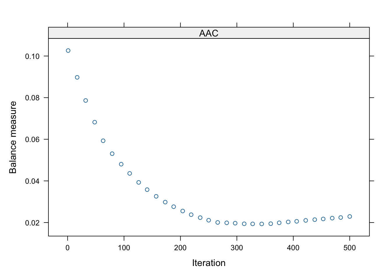
The plot showed the balance measure as a function of the number of iterations in the GBR algorithm. Model balance reached optimal around 350-ish iteration.
plot(pswt, plots = "optimize") # visualize the iteration process
| Version | Author | Date |
|---|---|---|
| 2739810 | Chun-Hui Lin | 2024-12-03 |
The average absolute correlation mean.wcor was minimized
at iteration iter 347, which means the specified
n.trees allowed GBR to explore sufficiently complicated
models.
summary(pswt) n ess max.wcor mean.wcor rms.wcor iter
unw 4000 4000.000 0.21633979 0.1034782 0.11887909 NA
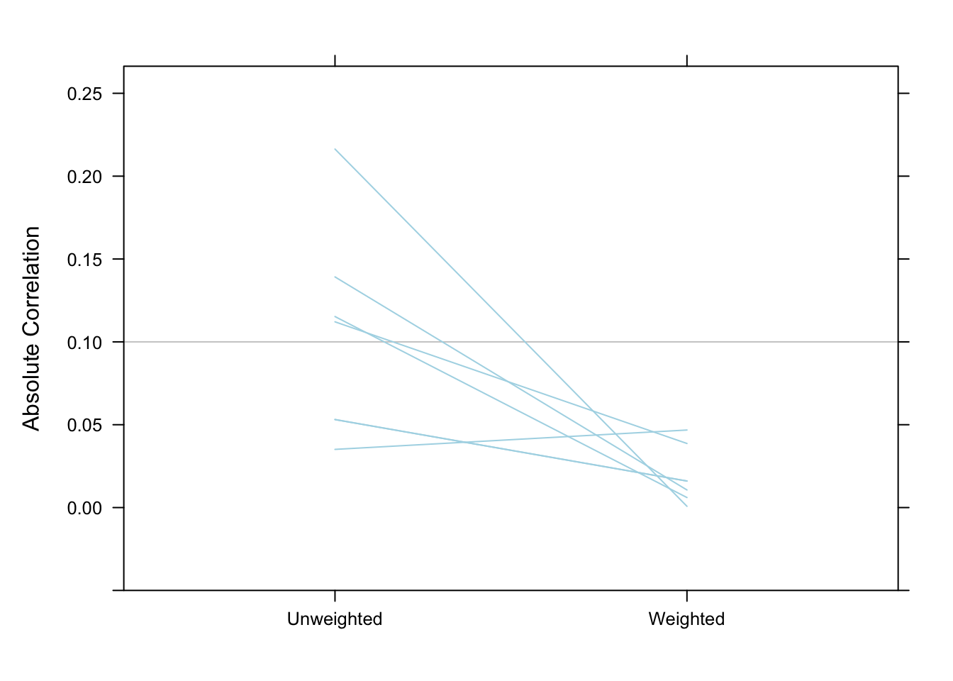
AAC 4000 3559.661 0.04680874 0.0192826 0.02492979 347Correlations between the exposure and potential confounders were all reduced to below 0.05 in the weighted data.
bal.table(pswt, digits = 3) unw wcor
sfs8p_0 0.115 -0.006
sati_0 0.139 -0.011
sp_sm_0 0.216 0.001
recov_0 -0.112 -0.039
subsgrps_n 0.035 -0.047
treatA 0.053 0.016
treatB -0.053 -0.016plot(pswt, plots = "es") # visualize the balance table
| Version | Author | Date |
|---|---|---|
| 2739810 | Chun-Hui Lin | 2024-12-03 |
Causal Effect
For every 1 point increase in baseline traumatic stress scale, the estimated substance frequency scale increased by 0.18 point.
tbl_regression(lm(sfs8p_3 ~ tss_0, dat),
               label = tss_0 ~ 'Baseline Traumatic Stress',
               estimate_fun = ~ style_sigfig(.x, digits = 3),
               pvalue_fun = ~ style_pvalue(.x, digits = 3)) %>%
modify_caption('**Unweighted Linear Regression**')| Characteristic | Beta | 95% CI1 | p-value |
|---|---|---|---|
| Baseline Traumatic Stress | 0.178 | 0.082, 0.274 | <0.001 |
| 1 CI = Confidence Interval | |||
After applying the propensity weights, the association between baseline traumatic stress and substance use at 3-month became insignificant.
# extract propensity weights
dat$wts = get.weights(pswt)

tbl_regression(lm(sfs8p_3 ~ tss_0, dat, weights = wts),
               label = tss_0 ~ 'Baseline Traumatic Stress',
               estimate_fun = ~ style_sigfig(.x, digits = 3),
               pvalue_fun = ~ style_pvalue(.x, digits = 3)) %>%
modify_caption('**Weighted Linear Regression**')| Characteristic | Beta | 95% CI1 | p-value |
|---|---|---|---|
| Baseline Traumatic Stress | 0.003 | -0.093, 0.098 | 0.957 |
| 1 CI = Confidence Interval | |||
sessionInfo()R version 4.4.0 (2024-04-24)
Platform: aarch64-apple-darwin20
Running under: macOS 15.3
Matrix products: default
BLAS: /Library/Frameworks/R.framework/Versions/4.4-arm64/Resources/lib/libRblas.0.dylib
LAPACK: /Library/Frameworks/R.framework/Versions/4.4-arm64/Resources/lib/libRlapack.dylib; LAPACK version 3.12.0
locale:
[1] en_US.UTF-8/en_US.UTF-8/en_US.UTF-8/C/en_US.UTF-8/en_US.UTF-8
time zone: America/Detroit
tzcode source: internal
attached base packages:
[1] stats graphics grDevices utils datasets methods base
other attached packages:
[1] gtsummary_2.0.3 twangContinuous_1.0.0 workflowr_1.7.1
loaded via a namespace (and not attached):
[1] gbm_2.2.2 xfun_0.47 bslib_0.8.0
[4] processx_3.8.4 lattice_0.22-6 callr_3.7.6
[7] vctrs_0.6.5 tools_4.4.0 ps_1.7.6
[10] generics_0.1.3 tibble_3.2.1 fansi_1.0.6
[13] highr_0.11 pkgconfig_2.0.3 Matrix_1.7-0
[16] gt_0.10.1 lifecycle_1.0.4 compiler_4.4.0
[19] stringr_1.5.1 git2r_0.33.0 getPass_0.2-4
[22] mitools_2.4 survey_4.4-2 httpuv_1.6.15
[25] htmltools_0.5.8.1 sass_0.4.9 yaml_2.3.10
[28] later_1.3.2 pillar_1.9.0 jquerylib_0.1.4
[31] whisker_0.4.1 tidyr_1.3.1 broom.helpers_1.17.0
[34] cachem_1.1.0 commonmark_1.9.1 tidyselect_1.2.1
[37] digest_0.6.37 stringi_1.8.4 dplyr_1.1.4
[40] purrr_1.0.2 forcats_1.0.0 splines_4.4.0
[43] labelled_2.13.0 rprojroot_2.0.4 fastmap_1.2.0
[46] grid_4.4.0 cli_3.6.3 magrittr_2.0.3
[49] cards_0.3.0 survival_3.7-0 utf8_1.2.4
[52] broom_1.0.7 withr_3.0.1 promises_1.3.0
[55] backports_1.5.0 rmarkdown_2.28 httr_1.4.7
[58] hms_1.1.3 evaluate_1.0.0 knitr_1.48
[61] haven_2.5.4 markdown_1.12 rlang_1.1.4
[64] Rcpp_1.0.13 xtable_1.8-4 glue_1.8.0
[67] DBI_1.2.3 xml2_1.3.6 rstudioapi_0.16.0
[70] jsonlite_1.8.9 R6_2.5.1 fs_1.6.4